Lab: Boyle’s Law

Overview

This lab is designed to demonstrate one of the fundamental laws of gas behavior, Boyle’s Law. This law is about the relationship between the pressure and volume of an ideal gas when the number of moles and the temperature are held constant. Furthermore, the law holds true regardless of the identity of the gas. Credit for the first publication about this law regarding gas behavior belongs to Robert Boyle who wrote up his results in 1662. You will use the Vernier Gas Pressure Sensor and a gas syringe to vary volume and measure pressure to generate data to graph in order to determine the nature of the proportion between the pressure and volume of a gas.

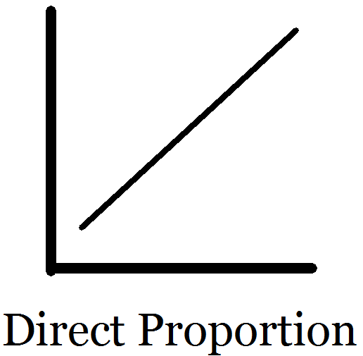
By collecting data and graphing it you will determine whether Boyle’s Law is a direct proportion or an inverse proportion. A direct proportion is one in which two variables are related in such a way that the value of the dependent variable (usually plotted on the y-axis) equals the independent variable (on the x-axis) multiplied by a constant. The graph of such a proportion has the form of a simple straight line and the equation for the line (in y = mx + b form) shows how one variable is multiplied by a constant (the slope of the line) to calculate the other. A sample graph of a direct proportion is shown at right.

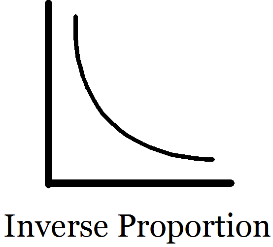
An inverse proportion is one in which two variables are related in such a way that the value of the dependent variable (y) equals a constant times the inverse of the independent variable (1/x). The graph of an inverse proportion has the form of a simple inverse curve and the equation of the curved line has the form y = m(1/x). The problem with this is that several functions have graphs that look a lot alike. When using real data from a lab it can be hard to be sure that the data are following the equation y = m(1/x) or y = m(1/x²). These two functions are hard to tell apart—try graphing them using a graphing calculator. In order to confirm that your data do follow a simple inverse proportion, just plot the inverse of your independent variable values versus the dependent variable. In other words, plug in the value of 1/x instead of x and graph it again. If it turns out to be a simple straight line, then you can confirm a simple inverse proportion.

Objective

This lab is designed to allow students to discover the nature of the proportion between the pressure and volume of a gas by collecting data and analyzing it using computer software. Students will determine whether Boyle’s Law is a direct proportion or an inverse proportion. They will also learn to do simple proportional calculations.

Materials

Safety

Pre-lab Exercises

Boyle’s Law is a useful proportion that can be put to work to answer questions about changes in volume and pressure.

If a gas’s pressure is reduced by half at constant temperature then its volume doubles. Here is how to use the Boyle’s Law proportion to calculate such changes.

First, let’s define the initial pressure and volume as P₁ and V₁ and the pressure and volume after a change as P₂ and V₂. According to Boyle’s Law:

P1V1 = k1     and     P2V2 = k2

Let’s assume those constants are the same (and they will be as long as we do not add or remove any gas or change the temperature). In that case:

P1V1 = P2V2

Now, here is a question we can answer using this proportional equation: What is the final volume of a gas when its pressure is reduced by half and its initial pressure is 1.0 atm and its volume is 5.0 L?

P1 = 1.0 atm          P2 = 0.50 atm                P1V1 = P2V2
V1 = 5.0 L            V2 = ?          (1.0 atm)(5.0 L) = (0.50 atm)(V2)

Solving for V₂ gives the answer 10 L. This is exactly what we expected based on the idea that this is an inverse proportion: when one variable is cut in half, the other doubles. Use this example to help you to answer the questions in the exercises below.

Exercises

Do the following exercises neatly on a separate piece of paper. Assume that temperature is constant for all of the changes described in these problems. Also, assume that pressure at the Earth’s surface is equal to 1 atm or 101.3 kPa.

All problems can be solved using the correct form of Boyle’s Law. This can be written as either PV = k or, more usefully, as P₁V₁ = P₂V₂.

Remember to record your observations in your lab notebook before you leave class.

1. Connect the LabQuest Mini to the computer and connect the Gas Pressure Sensor to it. Start the Logger software. Or, if using a Chromebook, search for “Graphical Analysis” and start it.
2. Set up data collection as follows:
   1. On the “Experiment” menu, select “Data Collection…” On Chromebooks, this is set up when you first start the software.
   2. Change Mode from “Time Based” to “Events with Entry”.
   3. Make the “Column Name” Volume and the units mL. Then click “Done”. (Pressure will be recorded using the SI unit of pressure, the kilopascal (kPa): 1 atm = 101.3 kPa.
3. Pull out the plunger of the syringe until the volume reads 5 mL. Read the volume at the bottom-most black ring on the rubber plunger where it touches the inside of the barrel.
4. Attach the syringe to the sensor by gently screwing it into place.
5. Right-click on the graph and select “Graph Options…” at the top of the menu that pops up. Things might look different on the Chromebook, but look for a way to edit the labels and range of the graph axes.
6. On the “Axes Options” tab change the box marked “Right” to 20. This sets the maximum value for the volume measurements which will not exceed 20 mL.
7. You are about to make measurements of pressure by manually choosing different volumes. The seal on the syringe is not perfect and at some pressures it may leak in or out. Pay attention to what you are doing and take steps to ensure that your data point is collected before significant leakage can take place.
8. If you have a lab partner then have one partner manage the syringe and have the other enter the data. Click the big green “Collect” button to begin.
   1. Move the piston of the syringe so that the volume is exactly 2.5 mL and hold it in place.
   2. Wait for the pressure reading to stabilize then click the “Keep” button. This will bring up a box in which you can enter the volume. Enter it.
   3. Repeat these steps at volumes of 5.0 mL, 10.0 mL, 12.5 mL, 15.0 mL, 17.5 mL, and 20.0 mL.
   4. Click the big red “Stop” button.
9. Once you have completed data collection, evaluate your data for quality. If you need help with this, ask your teacher. You are looking for data which exhibit a regular pattern as visualized on the graph in the data collection software. If necessary, collect another run of data. It does not take long and most students find this lab more satisfying when their data is of high quality.
10. Click the big “Save” button and write a descriptive name for the data file. Store it on your personal network drive. Alternatively, save it to the desktop and then email it to yourself or upload it to your personal document service.

Calculations and Graphing

Now that you have generated some data and taken a look at a graph of it on your screen you will put that data in Excel (or Google Sheets) to produce a well-formatted graph and perform an analysis to determine the exact nature of the proportion between the pressure and volume of a gas.

Note: Each individual student must make their own spreadsheet. One of the main values of this lab is the experience you gain in using spreadsheets to handle data and do calculations.

1. Highlight the data table on the data collection software screen. Copy by using Ctrl-C.
2. Paste the data into a spreadsheet program, leaving an empty row at the top to add labels. Label the column on the left “Volume (mL)” and label the column on the right “Pressure (kPa)”.
3. Insert a Scatter-plot graph of the data. For this graph, do not connect the data points with a line. In Google Sheets you may have to manually designate the x-axis and y-axis. Make sure volume is on the x-axis and pressure is on the y-axis. The option “use column A as labels” may be useful here. Label the axes and title the graph “Boyle’s Law”. Set the value for the minimum value on the x-axis to zero manually. This graph displays the ambiguous curve which you will analyze in the following steps to confirm that it is a simple inverse proportion. The online version of this lab has a link to a sample set of graphs.
4. Next you are going to let the spreadsheet calculate inverse volume values for all of your data points.
   Right-click the column heading for the column containing your Pressure data (probably where it says ‘B’) and select “Insert” from the menu that pops up and insert one new column to its left. Label this column “Inverse Volume (1/mL)”. In the cells of this column use a formula to calculate the inverse of the Volume data. One possible formula is “=A2^-1”. Copy the formula to all the cells in the column next to Volume data.
5. You are about to create a graph to confirm that this relationship is a simple inverse proportion. The first graph you made should have the appearance of data which are inversely proportional. By graphing P vs. 1/V you will see whether a straight line results. If it does then it will confirm the proportion as a simple inverse proportion that has the form PV = k. Create a scatter-plot of the 1/V and P data. As with the previous graph, do not connect the dots. Manually choose the x- and y-axes. Add axis labels and title the graph “Boyle’s Law, Inverse Volume”. Set the value for the minimum value on the x-axis to zero manually.
6. If the data do not turn out to be a nice straight line on your graph then consult with your teacher immediately to get help trouble-shooting.
7. Use the spreadsheet software to generate a line of best fit or trendline. In Google Sheets go to the “Customize” tab of the “Chart editor”. Under “Series” you will find the options you need. Be sure to show the equation on the graph. The slope of this line is the constant of the proportion (k).
8. As another way to confirm that this is an inverse proportion, which should have a constant value for P times V, follow these steps.
   1. To the right of the Pressure column of data add another column heading: “Pressure times Volume (kPa × mL)”.
   2. Set up a calculation of pressure times volume. A likely formula is “=A2*C2”. Copy the formula to all the cells in the column. The result of this calculation will be a constant for an inverse proportion.
   3. At the bottom of your column of P × V values calculate the average. Type: “=AVERAGE(D2:D7)” or use whatever data range is appropriate to your sheet.
9. Under the average, calculate the standard deviation. This is a measure of the degree to which data fluctuate above and below the average. If it is small relative to the size of the average then it supports the idea that the numbers in the average are reasonably constant. Calculate it automatically using a formula like this: “=STDEV(E2:E8)”, using the appropriate data range. Do not include the value of the average in this calculation.
10. In order to evaluate the size of the standard deviation, make another calculation below. Divide the value of the standard deviation by the value of the average. Format the cell as a percent. This gives a value called a Percent Error, which is not about mistakes but rather about how close data points are to one another. This is, in other words, a measure of precision. If it is less than about 5% then your data points can reasonably be said to be constant, within expected experimental error. Use a formula like this: “=E10/E9”, using cell references appropriate to your sheet. Format as a percent using the percent button at the top of the window.
11. Format your data table to turn it in by making the headings bold and adding borders around all cells. Make sure that you can see all data and both graphs on one single screen so that it will be easy for your teacher to see that you completed all of the required steps.
12. Create a Google Doc in which to answer the Post-lab questions. When you turn in your lab you will turn in both your spreadsheet document and your answers to the questions. To be clear, every student must work independently to write their own answers to those questions.

Post-lab Questions

Answer the following questions using complete sentences in a professional-quality typed document. Submit them along with your spreadsheet with neatly labeled data and graphs. Each student must do their own independent work.

1. What is the equation of the line for your second graph in the form y = mx + b? Identify each of the letters in [y = mx + b] with a quantity from the lab and clearly identify the units of each quantity. Give decimal values for the slope and y-intercept.
2. What is the average value of P × V?
3. What is your standard deviation for your P × V values and what is your percent error?
4. Comment on the precision of your data, any outlier data points, and physical reasons why your results are not perfectly constant for the values of P × V.
5. Check your data to answer the following questions:
   1. What happens to the pressure when you double the volume?
   2. What happens to the pressure when you cut the volume in half?
   3. What happens to the pressure when you triple the volume?
   4. What happens to the pressure when you cut the volume to one quarter?
6. What kind of proportion (direct or inverse) does your first graph of P vs. V look like? What does your graph P vs. 1/V tell you about the nature of the proportion between P and V?
7. Based on your graphs and the answers to the previous questions, should Boyle’s Law be written in mathematical form as PV = k (an inverse proportion) or as P/V = k (a direct proportion)? Justify your answer with direct references to your graphs and calculations.
8. According to the introduction, is Boyle’s Law valid if you change the temperature of the gas while also changing the volume? What do you think happens to the volume of a gas when you increase its temperature at constant pressure?
9. What do you think happens to the pressure of a gas when you decrease its temperature? Think about the air pressure in your car tires in the winter.