In this experiment you will determine the numerical value
of the equilibrium constant for the reaction:
Fe3+ + SCN– ⇌ FeSCN2+
This will be accomplished by measuring the equilibrium
concentration of the blood-red metal-complex ion
iron(Ⅲ) thiocyanate (FeSCN2+) with five different
initial concentrations of iron(Ⅲ) (Fe3+) and thiocyanate
(SCN–) ions.
The value of the equilibrium constant is calculated using
the equilibrium constant expression:
Keq = ĀĀ
[FeSCN2+]
[Fe3+][SCN–]
The value calculated for Keq will be the same,
within experimental error, for a variety of different
concentrations of the reactants and product.
The technique used to measure concentrations in this
experiment is spectrophotometry. Since iron(Ⅲ)
thiocyante is blood red in color (though its solutions at
low concentration appear orange) it absorbs light strongly
at the blue end of the visible spectrum. Specifically, its
wavelength of maximum absorption is 450 nm. You will use
absorption at this wavelength to find the equilibrium
concentration of FeSCN2+. By subtraction you
will calculate the concentration, at equilibrium, of
Fe3+ and
SCN–. Because
the stoichiometric ratios are 1:1 the concentration of the
product is the exact amount by which the concentration of
each reactant will be reduced. For example, if the measured
concentration of FeSCN2+ is 9.00 ×
10–5 M and the initial concentrations of
Fe3+ and
SCN– are
This gives a value for Keq of:
Keq = ĀĀ
(9.00 × 10⁻⁵)
Ā = 139
(9.10 × 10⁻⁴)(7.10 ×
10–4)
[Fe3+]0 =
1.00 × 10⁻³ M and
[SCN–]0 = 8.00
× 10–4 M
then the equilibrium concentrations will be:
[Fe3+]eq =
1.00 × 10⁻³ M – 9.00 ×
10–5 M = 9.10 × 10⁻⁴
M
[SCN–]eq = 8.00
× 10–4 M – 9.00 ×
10–5 M = 7.10 × 10⁻⁴
M
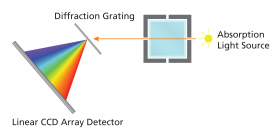
Vernier SpectroVis Instrument diagram
The value or 139 is similar to typical values usually found
in carrying out this experiment. Note that although the
value of Keq will be about the same (a typical
result is about a 15% variation) the concentrations of
reactants and products can be different. Each different set
of equilibrium concentrations is called an equilibrium
position.
Measuring [FeSCN2+]eq
This experiment depends on careful measurements of the
concentration of the colored complex ion’s
concentration. The initial concentrations of the reactants
are determined by the dilutions that take place when they
are mixed. If the concentration of FeSCN2+ is known, then
stoichiometry (see calculations above) can easily find the
equilibrium concentrations of the reactants. The question
then is, how do we measure the concentration of
FeSCN2+?
The answer is spectrophotometry. A spectrophotometer is an
instrument that measures the intensity of light after it is
passed through a colored solution. In order to use it the
intensity of the light source in the instrument is measured
with a colorless solution. The intensity of the light after
passing through the colored solution is then compared with
this ‘blank’ measurement to calculate the
amount of light absorbed, known as the absorbance. A
diagram of the instrument used in your lab is at right.
FeSCN2+ ion spectrum
A spectrophotometer can be used in a variety of ways. One
way to use it is to generate an absorbance spectrum. This
graphs the strength of light absorbance as a function of
wavelength. The image at right shows the absorbance
spectrum of the complex ion, FeSCN2+. The graph shows a region of the spectrum with
strong light absorbance centered on about 450 nm. The
spectrum shows almost no absorption above about 650 nm.
Since blue is absorbed and red is transmitted, the material
has a red appearance to our eyes. Because it is the blue
light that is absorbed, and because it is specifically the
light at 450 nm that is most strongly absorbed, this is the
wavelength of light that you will use to measure the
concentration of FeSCN2+.
page break
The absorption of light at a wavelength of maximum
absorption (λmax) is directly proportional
to the concentration of the colored substance. This
proportion is known at Beer’s Law: A = εbc
In this equation A represents absorbance (which has
no units). The concentration in mol/L is c, the path
length in centimeters is b (usually 1 cm), and
ε (the Greek letter epsilon) represents the
molar absorptivity constant in inverse molarity and inverse
cm (M–1cm–1). This
constant relates the
Sample Results for Part I
Reference Solution Concentrations:
Before
Equilibrium
Fe3+
ĀĀ+ĀĀ
SCN–
ĀĀ⇌ĀĀ
ĀĀĀĀĀĀ
After
Equilibrium
Fe3+
ĀĀ+ĀĀ
SCN–
ĀĀ⇌ĀĀ
FeSCN2+
Schematic showing how the big difference in initial conc. of reactants leads to a predictable concentration of the product
concentration of a solution to the amount of light
absorbed at a specific wavelength. It is a direct proportion
and so if a series of solutions with a known concentration
are placed into the spectrophotometer to measure their
absorbances it is possible to determine the value of ε.
Once you have a value for ε you can measure the
absorbance of a solution with an unknown concentration and
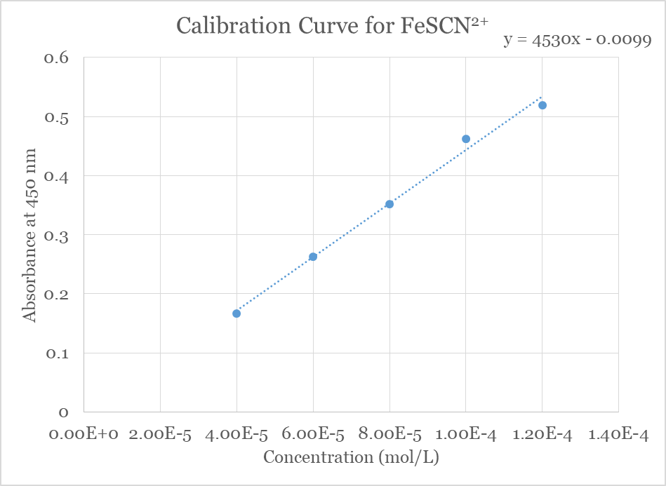
use it to calculate the concentration. For this experiment
you will need to have a series of at least five solutions
with known concentrations of FeSCN2+. By entering these
concentrations (x-axis) and the measured absorption of each
one at 450 nm (y-axis) you will construct a graph and use it
to determine the slope of the best-fit line for the five data
points. Usually a spreadsheet program or a graphing
calculator simplifies this process. A graph of sample data is
shown below demonstrating the construction of what is called
a calibration curve and showing the equation of the line. The
slope of this line is equal to ε.
The problem remains, however, of how to establish the
concentration of a solution of FeSCN2+ independent of
spectrophotometric measurements. It turns out to be quite
straightforward. The idea is to arrange the concentrations
of the reactants in such a way that regardless of the value
of the equilibrium constant we can make a valid assumption
about the concentration of FeSCN2+. This is done by
putting Le Châtelier’s Principle into practice.
Le Châtelier’s Principle is the idea that a
system at equilibrium will respond to stresses placed on
that equilibrium by changing reactant and product
concentrations in such a way as to minimize the stress. For
example, if the concentration of one reactant is increased
then when a new equilibrium position is established the
concentrations of both reactants will decrease while the
concentration of products will increase. This uses up the
added reactant and minimizes the stress on the equilibrium.
In this experiment the series of five solutions with a
known concentration of FeSCN2+ will be made by using a
huge excess of Fe3+
ions and a very small concentration of SCN– ions. In this way
the initial concentration of SCN– ([SCN–]0) is
reduced effectively to zero at equilibrium and is
stoichiometrically converted into FeSCN2+. This is illustrated
schematically at right. The main idea can be expressed
symbolically like this:
[SCN–]0 =
[FeSCN2+]eq
In summary: In Part I you will measure volumes of
high-concentration iron(III) (Fe3+) and low-concentration
thiocyanate (SCN–) and mix them to
make five reference solutions. In the reference solutions
the equilibrium concentration of the complex ion will be
assumed to be equal to the initial concentration of the
thiocyanate ion. The initial concentration of SCN– was so low that it is
stoichiometrically converted. There is a difference of a factor of about a thousand between the concentration of the Fe3+ and the SCN– in order to guartantee this assumption will be true. These five reference
solutions will be used to establish a direct proportion
between absorption of light at 450 nm and molar
concentration of the complex ion (FeSCN2+). By doing so you will
make it possible to measure the equilibrium concentration
of the complex ion in the trials designed to be used to
measure the value of the equilibrium constant.
In Part II you will mix iron(III) and thiocyanate
solutions with roughly similar concentrations. Neither
reactant will be completely converted into the product in
these solutions so that both reactants and the product will
have significant and comparable concentrations at
equilibrium. By measuring the absorbance of these solutions
at 450 nm you will measure the molar concentration of the
complex ion. Then, by using stoichiometry, you will
calculate the concentration of the two reactants at
equilibrium based on the fact that all of the product
molecules exist due to the consumption of some of the
reactant molecules.
page break
Ā
Objectives
Determine the Beer’s Law constant for
FeSCN2+
Measure the value of Keq for five different
sets of initial concentrations of Fe3+ and
SCN– for the reaction: Fe3+ +
SCN–
⇌ FeSCN2+.
(Part II) 2.0 × 10⁻³ M
potassium thiocyanate (KSCN)
solution
distilled water
spectrophotometer capable of providing absorbance at
450 nm
11 cuvets (1 for a blank and 10 for the reaction mixtures)
15 50-mL beakers (one for each stock solution and one for each mixture)
marker to label beakers
syringes for measuring solutions
or graduated pipets and pipet bulbs
disposable pipets for transfers
lint-free wipes
Note: the iron(III) nitrate solutions use 1.0 M
nitric acid (HNO3)
to dilute the stock solution. This
reduces the natural color of the iron(III)
ions.
Safety
The following list does not cover all possible hazards,
just the ones that can be anticipated. Move slowly and
carefully in the lab: haste and impatience have caused more
than one accident.
Always leave stock solution bottles tightly closed when
not in immediate use!
As always, wash hands before leaving the lab, eating,
or drinking, or going to the bathroom.
Wear chemical splash goggles, gloves, and a
chemical-resistant apron.
Iron(III) nitrate is a skin and tissue irritant; it is
corrosive and toxic, and causes stains. Use care in
handling the solution.
Nitric acid (HNO3) is corrosive and toxic.
This chemical is used in making the iron(III) nitrate
solutions and adds to their toxicity and corrosiveness.
Potassium thiocyanate (KSCN) is toxic by ingestion. Avoid contact
with eyes and skin.
All solutions used in this lab must be collected for
hazardous waste disposal. None of the reactants or products
may be dumped into the sewer system.
Collect all waste in the designated bottle by pouring the
solution out of the cuvet, rinsing the cuvet by filling it
once with tap water and pouring it into the bottle, and the
closing the bottle again. Use the funnel provided to make
splashing outside the bottle less likely.
Procedure
The most time-consuming part of the lab is mixing the ten solutions you need. Part I requires 5, with 10 volume measurements. Part II requires 5, with 14 volume measurements. Since precision is desirable you may want to make all of the solutions at once, even though the procedure splits them into their own respective sections. The spectroscopic measurements can be accomplished relatively quickly.
Part I
In this part of the lab you will collect absorbance vs. concentration data for the complex ion (FeSCN2+) in order to establish a relationship between absorbance and concentration at equilibrium. You will use the data to make a Beer’s Law plot; the slope of the best-fit straight line for this plot is the constant of the proportion between absorption and concentration.
Obtain two small beakers. Label one “0.2 M
Fe(NO3)3” and
label the other “2 x 10⁻⁴ M
KSCN”. These are the Reference solutions.
Into the Fe(NO3)
3 beaker collect about 50 mL of the
reference stock solution (0.2 M).
Into the KSCN beaker
collect about 30 mL of the reference stock solution (2 x
10–4 M).
You will need 5 50-mL beakers into which you can
measure out the amounts of each solution required. Label
them Ref. 1 - 5.
Mix the solutions to make the reference solutions
according to the information in the table. Using a separate
syringe or pipet for each solution, measure the amounts of each one
needed into the labeled beakers. Do the necessary
calculations to fill in the rest of the table.
In the following table, calculate and then fill in the
initial concentration of each of the reactants in the space
provided. The solutions are designed to have such a large concentration of iron(III) ions that all of the thiocyanate ions will be used up at equilibrium. In this was we can assume that the equilibrium concentration of the complex ion (FeSCN2+) is equal to the initial concentration of thiocyanate.
Part I: Reference Solution Volumes
Solution
Volume of
0.200 M Fe(NO3)3
Volume of
2.0 × 10⁻⁴ M KSCN
Initial Conc.
of Fe(NO3)3 or
[Fe(NO3)3]0
Initial Conc.
of KSCN or [KSCN]0
Equilibrium Conc.
of FeSCN2+
([FeSCN2+]eq = [KSCN]0)
Ref. Soln. 1
8.0 mL
2.0 mL
Ā
Ā
Ā
Ref. Soln. 2
7.0 mL
3.0 mL
Ā
Ā
Ā
Ref. Soln. 3
6.0 mL
4.0 mL
Ā
Ā
Ā
Ref. Soln. 4
5.0 mL
5.0 mL
Ā
Ā
Ā
Ref. Soln. 5
4.0 mL
6.0 mL
Ā
Ā
Ā
When you are done with the syringes, take them apart and rinse well to clean them for re-use. Pipets may simply be rinsed well. Set aside to dry.
Each reference solution will need to be measured in the spectrophotometer. Stir each one carefully so that no cross-contamination occurs. Then fill a cuvet with each solution using a disposable pipet, capping them after they are full. They have a capacity of about 3 mL. Be careful to keep track of which cuvet has which reference solution in it!
Fill a cuvet with a blank solution consisting of about
3 mL of the 0.200 M Fe(NO3)3 solution.
Place it into the spectrophotometer with the flat, smooth
sides facing the white circle and triangle.
Plug the SpectroVis Plus unit into the USB port of the
computer and start the Logger Lite or Logger Pro software.
Or if you are using a Chromebook, use the search function
to find “Vernier Spectral Analysis”.
Calibrate the Spectrometer by finding this function in
your software. This step is critical because it provides
the baseline for brightness measurements to determine the
absorption of light.
A dialog box will pop up to inform you that the lamp is
warming up. Do not skip this step, it only requires 90
seconds.
Once Calibration is complete, click OK.
Set up data collection so that you collect Absorbance vs. Concentration (Beer’s Law) data. Choose 450 nm as the selected wavelength. Once you start collecting data you will need to press the “Keep” button to record a data point. For each one you have to enter the concentration. This is the equilibrium concentration of the complex ion ([FeSCN2+]eq), which you calculated in the table above. If you have not calculated them yet then just write down the absorbance values for each solution, which will appear on your screen when you insert the sample into the spectrophotometer.
When you finish collecting data press the “Stop” button. Copy and paste your data into a spreadsheet program for further analysis. Do not close the software or unplug the spectrophotometer! You still need it set up exactly as it is for Part II.
In the spreadsheet program create a graph of concentration vs. absorbance and set it up following the example in the introduction in this lab handout. You will need to label the axes, give your graph a title, and get it to produce a line of best fit (a trendline) and to display the equation of the line on the graph. The slope of the line is the molar absorptivity constant, epsilon (ε). You will use it to calculate the concentration of FeSCN2+ from absorbance measurements in Part II.
Once you have confirmed with your teacher that you have collected the data you need you may dispose of the contents of the cuvets. All waste liquids are to be collected in a bottle designated by your teacher. Use the provided funnel to ensure all liquid gets in the bottle. When you finish, take out the funnel and put the cover back on the bottle.
page break
Part II
In this part of the lab you will measure the absorbance of five solutions with different initial concentrations of reactants. The absorbance can be used to calculate the equilibrium concentration of the complex ion ([FeSCN2+]eq), which in turn will be used to calculate [Fe3+]eq and [SCN–]eq
Obtain two small beakers. Label one “2 × 10⁻³ M
Fe(NO3)3” and
label the other “2 x 10⁻³ M
KSCN”. These are the Experiment solutions.
Into the Fe(NO3)
3 beaker collect about 30 mL of the
experiment stock solution (2 × 10⁻³ M).
Into the KSCN beaker
collect about 25 mL of the experiment stock solution (2 x
10–3 M).
You will need 5 50-mL beakers into which you can
measure out the amounts of each solution required. Label
them Exp. 1 - 5.
Mix the solutions to make the experiment solutions
according to the information in the table. Using a separate
syringe or pipet for each solution, measure the amounts of each one
needed into the labeled beakers. Do the necessary
calculations to fill in the rest of the table.
In the following table, calculate and then fill in the
initial concentration of each of the reactants in the space
provided.
Part II: Experiment Solution Volumes
Solution
Volume of
2.0 × 10⁻³ M Fe(NO3)3
Volume of
2.0 × 10⁻³ M KSCN
Volume of
distilled water
Initial Conc.
of Fe(NO3)3 or
[Fe(NO3)3]0
Initial Conc.
of KSCN or [KSCN]0
Exp. Soln. 1
5.0 mL
2.0 mL
3.0 mL
Ā
Ā
Exp. Soln. 2
5.0 mL
3.0 mL
2.0 mL
Ā
Ā
Exp. Soln. 3
5.0 mL
4.0 mL
1.0 mL
Ā
Ā
Exp. Soln. 4
5.0 mL
5.0 mL
0 mL
Ā
Ā
Exp. Soln. 5
4.0 mL
6.0 mL
0 mL
Ā
Ā
When you are done with the syringes, take them apart and rinse well to clean them for re-use. Pipets may simply be rinsed well. Set aside to dry.
Each experiment solution will need to be measured in the spectrophotometer. Stir each one carefully so that no cross-contamination occurs. Then fill a cuvet with each solution using a different disposable pipet for each solution. Cap them after they are full. They have a capacity of about 3 mL. Be careful to keep track of which cuvet has which experiment solution in it!
Do not recalibrate your spectrophotometer! It should remain in the state it was in when you finished collecting the reference data. In fact, collect the data for Part II immediately after completing your data collection for Part I.
Insert each experiment sample into the spectrophotometer. The readout on the screen will show the absorbance at 450 nm. You just need to write this number down; write it in the data table provided below. Every lab group member should write down the data so no one is depending on getting the data later. There is no graph to be made for this part. Each point you collect here will be mapped onto the graph based on your Part I data. This will enable you to calculate the equilibrium concentrations of the reactants and product.
Fill in the table below by calculating the initial concentrations, recording your absorbance measurements, and calculating the equilibrium concentrations and the value of the equilibrium constant. This can be easily done in a spreadsheet, which will prepare you for your lab report. Be sure to do these calculations before you leave the lab. Here is how to do the calculations:
To use absorbance to calculate [FeSCN2+]eq:
A = absorbance measurement, ε = molar absorptivity constant, c = conc. in mol/L
c = A/ε
(the path length is 1 cm so that has been deliberately left out)
To use [FeSCN2+]eq to calculate [Fe3+]eq:
[Fe3+]0 – [FeSCN2+]eq = [Fe3+]eq
this is because, stoichiometrically, every unit of FeSCN2+ that is made uses up one unit of Fe3+
To use [FeSCN2+]eq to calculate [SCN–]eq:
[SCN–]0 – [FeSCN2+]eq = [SCN–]eq
this is because, stoichiometrically, every unit of FeSCN2+ that is made uses up one unit of SCN–
To calculate Keq:
Since the reaction is:
Fe3+ + SCN– ⇌ FeSCN2+
Keq = ĀĀ
[FeSCN2+]eq
[Fe3+]eq[SCN–]eq
Once you have confirmed with your teacher that you have collected the data you need you may dispose of the contents of the cuvets. All waste liquids are to be collected in a bottle designated by your teacher. Use the provided funnel to ensure all liquid gets in the bottle. When you finish, take out the funnel and put the cover back on the bottle.
The following table may be filled in by hand but it is highly recommended that you enter the data directly into a spreadsheet to handle your calculations automatically and to speed the formatting of your results for your lab report.
Part II: Calculating Concentrations
Solution
[Fe(NO3)3]0
[KSCN]0
Absorbance
[FeSCN2+]eq
[Fe3+]eq
[SCN–]eq
Keq
Exp. Soln. 1
Ā
Ā
Ā
Ā
Exp. Soln. 2
Ā
Ā
Ā
Ā
Exp. Soln. 3
Ā
Ā
Ā
Ā
Exp. Soln. 4
Ā
Ā
Ā
Ā
Exp. Soln. 5
Ā
Ā
Ā
Ā
page break
The Formal Lab Report
Each indiviual student will write and submit an independently written formal lab report.
Introduction
A definition of chemical equilibrium
the equilibrium constant expression.
The chemical equation whose equilibrium you are
investigating: Fe3+
+ SCN–
⇌ FeSCN2+
The method, briefly, by which you determined the
equilibrium concentration of FeSCN2+.
The purpose of the lab, to calculate the
value of the equilibrium constant for the formation of the
FeSCN2+ ion.
Procedure
While giving a brief overview of the steps taken to
complete the experiment, be sure to include the following:
Why are the concentrations of Fe3+ and
SCN– so different in size for
part 1 of the experiment where you are creating the
calibration curve?
Why are the concentrations of Fe3+ and
SCN– similar in size in part 2
where you are determining unknown equilibrium
concentrations of FeSCN2+?
Data and Graphs
The data used for the determination of the Beer’s Law
constant for FeSCN2+.
The graph of your calibration curve.
A data table with the following headings:
Sample #, [Fe3+]
0, [SCN–]0, Absorbance, [FeSCN2+]eq, [Fe3+]
eq, [SCN–]eq, Keq
The data table should
include an average Keq value, the standard
deviation (as can be calculated using a spreadsheet), and a percent
error (caculated as (std. deviation)/(average value)
× 100%). Note: no other values can or should be averaged.
Sample Calculations
One instance of calculating equilibrium concentration
of FeSCN2+ using
Beer’s Law.
One instance of calculating [Fe3+]eq and
[SCN–]eq.
One instance of calculating the value of
Keq.
Analysis
The average value of Keq, your standard
deviation, and percent error.
Comment on factors which could have led to variation in
your result. The spectrophotometer’s measurements may
be assumed to be precise and accurate enough to be
neglected in your answer.
Did the value of Keq vary as you increased the initial concentration of KSCN? Why or why not?
Does the level of variation in your results raise the
question of the validity
of the name constant for Keq? Explain.
Based on the size of your determined value for
Keq does this reaction favor products or
reactants? Explain.
Conclusion
Comment on the educational experience of carrying out this
experiment.
.Thiocyanate.Visible.Spectrum.png)